Spline Approximation (Mathematics)

The goal of spline approximation has already been explained in the previous article „Spline Approximation (Introduction)„.

This article will cover the mathematics behind this approximation and develop an approach. If you do not care about the mathematics, just skip this article and read the Spline Approximation (Cookbook)“, that will come soon.

Spline Interpolation

We have points

$(x_0, y_0), (x_1, y_1), \ldots, (x_n, y_n)$

such that

(0.1) $x_0 < x_1 < x_2 < \ldots < x_n$

and want a function f such that

$(1)\thickspace \bigwedge_{i=0}^n f(x_i) = y_i$

and f is continuous. Usually the requirement goes further, so the first and second derivative should also be continuous too.

The way this is accomplished is by defining cubic polynomials $f_j$ on each interval $[x_j, x_{j+1}]$ such that

$(2)\thickspace \bigwedge{j=1}^{n-1} f'_{j-1}(x_j)=f'_j(x_j)$

$(3)\thickspace \bigwedge{j=1}^{n-1} f''_{j-1}(x_j)=f''_j(x_j)$

Now this gives us $4n$ unknowns and together with the initial condition $2(n-1)+2n$ equations. So this is underdetermined, which is usually resolved by adding two more or less arbitrary conditions. A lot of material can be found about this in the internet, in papers and in books.

Spline Approximation

Now a more interesting case is that we actually have much more given points than spline intervals. So we have interval borders at points

$x_0,\ldots,x_n$

and we have given pairs

$(\xi_1,\eta_1), \ldots, (\xi_N, \eta_N)$

with $N$ much larger than $n$ . The exact condition will become clear later, but for the time being it should be assumed, that $N$ is meant to be much larger than $n$ . The values $\xi_i$ may contain duplicates, but in that case the number of different values for $\xi_i$ should also be much larger than $n$ .

Btw. this is nothing new. Papers about this topic exist, but it is not as commonly found on the internet as the interpolation.
From here onwards, it is assumed, that the intervals all have the same length, i.e. there is some positive real number $h$ such that $x_i=x_0+i*h$ for all $i$ .

So we want the conditions (2) and (3) to be fullfilled and a weaker condition

$(1a)\thickspace \bigwedge_{j=1}^{n-1} f_{j-1}(x_j)=f_j(x_j)$

and we want $f(\xi_i)$ to be „somewhat close“ to $\eta_i$ for all points $(\xi_i, \eta_i)$ . More precisely it should be as close as possible on „average“, where the quadratic mean is used as „average“. That is common practice, allows for smooth formulas and works. To just minimize the quadratic mean, taking the square root and dividing by $N$ can be ommitted. So this can be made explicit by requiring the sum of the squares of the differences to be minimal i.e.

$(4)\thickspace \sum_{i=1}^N (f(\xi_i)-\eta_i)^2 \text{ is minimal}$

Btw. this can be done perfectly well with complex valued functions, we just need to replace the squares by the squares of the absolute values. So on the „ $\eta$ -side“ we can have complex numbers. Allowing complex numbers on the „ $\xi$ -side“ is a bit more involved, because being differentiable twice implies that the function would be holomorphic, so combining different functions is impossible. And even complex valued functions would become non continuous at the glue lines if we simply apply them to the whole complex plain. So, for the time being, real numbers are assumed.

Now the valid spline functions on the given set of intervals obviously form a vector space. Conditions (1a), (2) and (3) remain valid when we multiply by a constant or add two such functions. Having $4n$ parameters and $3(n-1)$ independent conditions, its dimension should be $n+3$ . This can be proved by induction. For $n=1$ any cubic polynomial (of degree $\le 3$ ) can be used. These form a 4-dimensional vectorspace. Assuming that for $n$ subintervals the valid spline functions form a vector space of dimension $n+3$ , then for $n+1$ subintervals the additional subinterval $[x_n, x_{n+1}]$ is added. In this subinterval, the function can be expressed as

$f(x)=a+b(x-x_n)+c(x-x_n)^2+d(x-x_n)^3\text{.}$

Conditions (1a), (2) and (3) already fix the values for $a$ , $b$ and $c$ , while $d$ can be choosen freely. Thus the dimension is exactly one higher and the assumption is proved.

Now a basis for this vector space should be found. Ideally functions that are only non-zero in a small range, because they are easier to handle and easier to calculate.

This can be accomplished by a function that looks like this:

Note that this is not the Gaussian function curve, which never actually becomes zero. The function we are looking for should actually be 0 outside of a given range. So assuming it is $f(x)=0$ for $|x| > A$ and $f(x)>0$ for $|x| < A$ for some constant $A>0$ . This implies that the first and second derivative are $0$ for $x=-A$ . So in the subinterval starting at $-A$ it needs to be a cubic polynomial of the form $a(x+A)^3$ . So further subintervals are needed to return to $0$ . For reasons of symmetry there should be a subinterval ending at $A$ in which the function takes the form $a(A-x)^3$ . Using a third subinterval $[-B, B]$ for the whole middle part would imply that this has to be an even function, thus of the form $g(x)=b+cx^2$ . $b$ could be determined as $b=a(A-B)^3-cB^2$ . According to the first derivative condition we would have $3(A-B)^2 = g'(-B) = -2cB$ , thus $c=-\frac{3(A-B)^2}{2B}$ . According to the second derivative condition we would have $6(A-B)=g''(-B)=2c=-\frac{3(A-B)^2}{B}$ thus $B=3(A-B)$ thus $B=\frac{3}{4}A$ Since subintervals of equal length are required, this is not adequate.

Using a total of four subintervals actually works. In this case for the subinterval $[-B,0]$ four conditions are given to determine the four coefficients of the cubic function.

For readability it will be assumed that $A=2$ and $B=1$ , so the subintervals are $[-2,-1], [-1, 0], [0,1], [1,2]$ . The function can be choosen as

$f(x)= \begin{cases} 0 &\text{for } x \le -2\\ (x+2)^3&\text{for } -2 < x \le -1 \end{cases}$

Now

$f(x)=a+b(x+1)+c(x+1)^2+d(x+1)^3$

needs to be defined in [-1, 0] such that

$f(-1)=1$

$f'(-1)=3$

$f''(-1)=6$

$f'(0)=0$

Thus $a=1$ , $b=3$ , $c=3$ and

$0=f'(0)=b+2c+3d=9+3d$

Thus $d=-3$ .

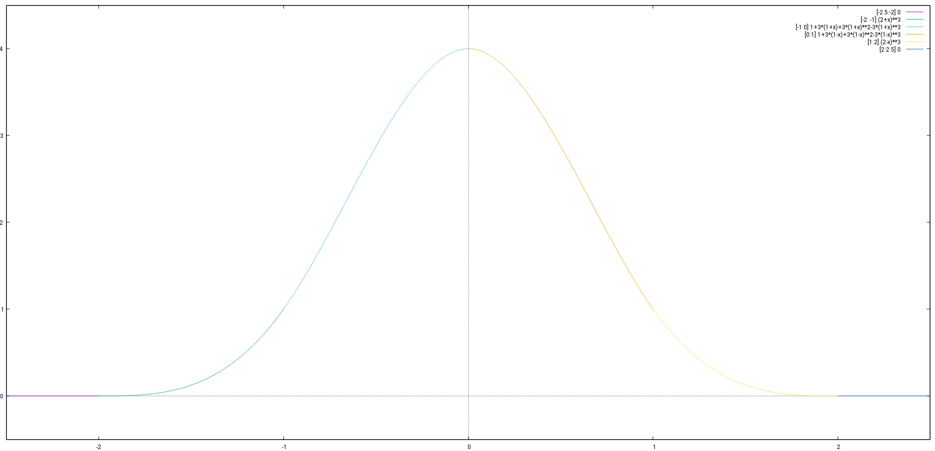
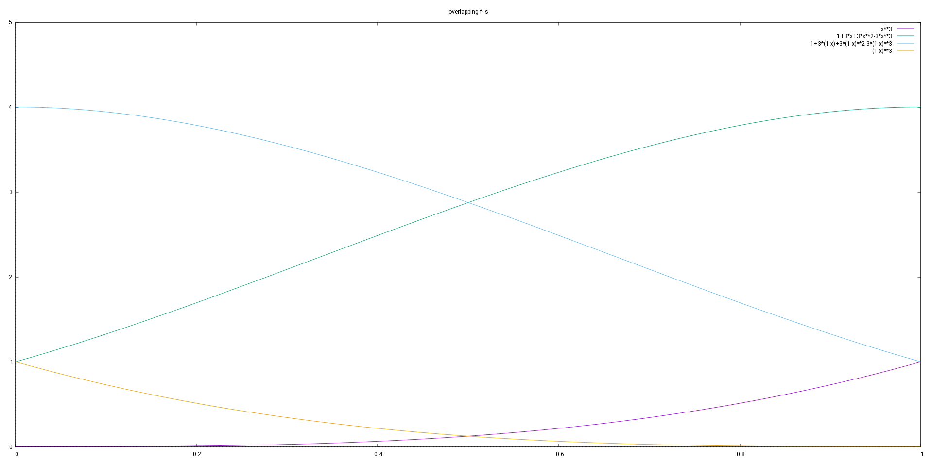
So the prototype function is

$(5)\thickspace f(x)= \begin{cases} 0 &\text{for } x \le -2\\ (x+2)^3&\text{for } -2 < x \le -1\\ 1+3(x+1)+3(x+1)^2-3(x+1)^3&\text{for } -1 < x \le 0\\ 1+3(1-x)+3(1-x)^2-3(1-x)^3&\text{for } 0 < x \le 1\\ (2-x)^3&\text{for } 1 < x \le 2\\ 0&\text{for } x > 2 \end{cases}$

A base for this vector space can be found using functions $f_i$ for $i=-3\ldots n-1$ . For readability purposes we define

$x_{j}=x_0+jh$

even for negative $j$ and $j>n$ .

The functions $f_i$ are defined such that such that

$f_i(x)=f\left(\frac{x-x_i}{h}\right) \text{ for } i=-1,\ldots,n+1$

These functions fulfill conditions (1a), (2) and (3), because they inherit that from $f$ .

By induction it can be proved that they are linear independent. It is true for $\{f_{-1}\}$ alone. If it is true for $\{f_{-1},\ldots,f_{i-1}\}$ it is also true for $\{f_0,\ldots,f_i\}$ , because

$f_i\left(x_i+\frac{3}{2}h\right) >0$

and

$\bigwedge_{j=-1}^{i-1}f_j\left(x_i+\frac{3}{2}h\right)=0\text{.}$

Since

$\{f_{-1},\ldots,f_{n+1}\}$

contains exactly $n+3$ elements, it is a vector space basis.

That means that we are searching for a function

$(6)\thickspace g(x) = \sum_{i} a_i f_i(x)$

such that the minimality condition (4) holds.
This is accomplished by filling (6) into (4) and calculating the partial derivatives with respect to each $a_i$ :

$(4a)\thickspace S(a_{-1},\ldots,a_{n+1}) = \sum_{j=1}^N \left(g\left(\xi_j\right)-\eta_j\right)^2$

$= \sum_{j=1}^N ( \sum_{i} a_i f_i(\xi_j)-\eta_j)^2$

Thus

$(4b) \thickspace\bigwedge_{k=-1}^{n+1} 0 &= \frac{\partial}{\partial a_k}\sum_{j=1}^N \left(g\left(\xi_j\right)-\eta_j\right)^2$

$= \frac{\partial}{\partial a_k}\sum_{j=1}^N \left( \sum_{i} a_i f_i\left(\xi_j\right)-\eta_j\right)^2$

$=\sum_{j=1}^N \left(2 f_k\left(\xi_j\right)\left( \sum_{i} a_i f_i\left(\xi_j\right)-\eta_j\right)\right)$

$=2\sum_{i} a_i \sum_{j=1}^N f_k\left(\xi_j\right)\left( f_i\left(\xi_j\right)-2\sum_{j=1}^N \f_k\left(\xi_j\right)\eta_j\right)$

So it comes down to solving the linear equation system

$\sum_{i=-1}^{n+1} a_i \sum_{j=1}^N f_k\left(\xi_j\right) f_i\left(\xi_j\right) = \sum_{j=1}^N f_k\left(\xi_j\right)\eta_j\thickspace\text{ ~ for }k=-1,\ldots,n+1$

This can be solved using a variant of the Gaussian elimination algorithm. Since this is a numerical problem, it is important to deal with the issue of rounding. Generally it is recommended choosing the pivot element wisely.
In this case the approach is chosen to iterate through the columns. For each column the line is chosen, in which the element in that column has the largest absolute value relative to the cubic mean of the absolute values of the other entries in the line.

When actually using the spline function a lot, it is probably a good idea to consolidate the linear combinations of different $f_i$ s within each subinterval into a cubic polynomial of the form

$f(x)=a+b(x-A)+c(x-A)^2+d*(x-A)^3.$

This can be based on the starting point of the interval or the end point or some point in the middle, probably the arithmetic mean of the interval borders. These choices of A have some advantages, because it makes the terms that need to be added smaller in terms of absolute value. Since the accurate end result is anyway the same, this helps avoiding rounding errors, that can go terribly wrong when adding (or subtracting) terms with large absolute values where the result is much smaller than the terms. So the arithmetic mean of the subinterval borders might be the best choice.

The actual formulas and a program will be added in one or two articles in the near future.

Spline Interpolation

Spline Approximation

Links

Beteilige dich an der Unterhaltung

Schreibe einen Kommentar

Antworten abbrechen